SIFT and Project 2: SIFTNet
Created by Shenhao Jiang and John Lambert on 24th, Sept, 2019.
Having received a ton of questions on “what is going on?” and “how do I start?” during the office hours and on Piazza, I’ll try explaining the basic concepts of SIFT here and also provide some guide on approaches to start building the network. Also, I’ll try my best to incorporate some hints on how you can use PyTorch to achieve the goals. I decided to work on this tutorial just 10 min ago, so bear with me for some of the wordings :-)
Scale Invariant Feature Transformation (SIFT)
All of this starts with the idea of image gradients: the layer you have implemented earlier and the Ix and Iy thing: these values tell you how much the current pixel is changing relative to my neighbors. You are probably use to taking derivatives of continuous functions, but for discrete functions/signals like 2d image arrays, we’ll use finite difference approximations of the derivative, such as the forward difference or central-difference that you have probably seen in calculus. Here’s an example of how to compute partial derivatives with respect to the x and y directions for a small 3x3 patch:
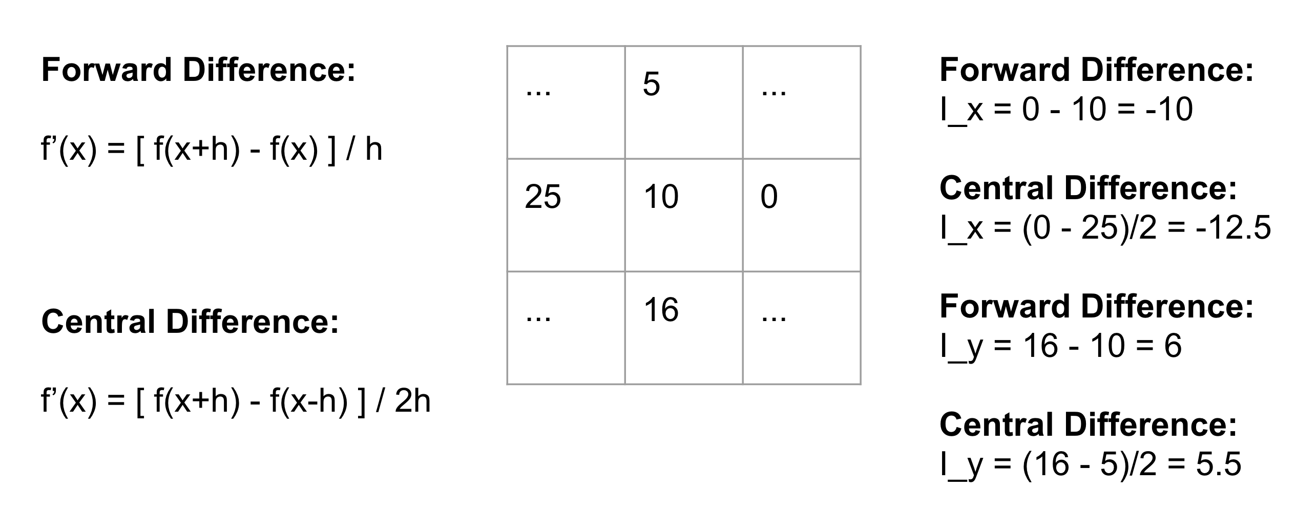
It turns out that an easy way to compute an partial derivative (by central difference) at each pixel is to convolve the image with a filter like
K = [
 [1,0,-1],
 [2,0,-2],
 [1,0,-1]
]
You’ll end up with a feature of this pixel, derived from info in the local image patch. So for each of the pixels in your image, there is this set of values: how much I’m changing in and directions.
Now consider a patch of pixels, say 8x8, then every one of the 64 pixels has an and , and if we think about and as forming a vector magnitude, then we can say things like: for pixel a, it is mainly pointing towards the direction of , where and represent the unit vectors in and directions; what does this mean? How much does the gradient contribute to and directions, right? And the contribution is essentially the projection onto the x and y axes. On the other hand, if our coordinate system consists of 8 directions/axes, we could do similar things like projecting the gradient vector onto these 8 directions and see which direction this vector is contributing the most.
If we divide the 8x8 patch to 4 sub-regions (4x4 each), then for every sub-region, we should be able to tell one idea: on direction 1, how much contribution I received from this sub-region in total, on direction 2 how much contribution, etc … and the end result is (meaning for sub-region ), and concatenating for 4 subregions/subgrids, we have a thing called a SIFT feature descriptor.
Why does this work as a feature? Well, let’s consider the following mini-example (sorry for the bad drawing; here are 2 doors):
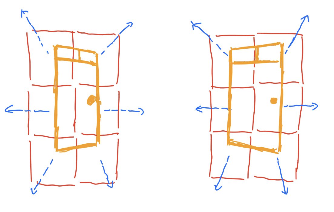
So the orange shape represents a door (the left and right images mean we take the images of the door from different angles), and red squares mean the 6 sub-regions, and suppose the blue vectors give the most contributing directions of this patch. Then if we concatenate the 6 vectors together from the left image, we can tell that for a door, we end up with a descriptor where the first region direction is pointing to top-left, second pointing to top-right, etc… Let’s say we take an image of the door from another angle (the image on the right), although the directions may differ a little bit, but the concatenated vectors are similar right?
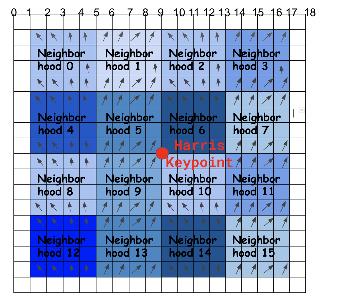
You should already have computed keypoints with your Harris Corner detector (red circle below). Now, you’ll seek to describe this keypoint with a ``descriptor’’. The SIFT descriptor will combine information about local neighborhoods in a 16x16 patch around the keypoint. In total, you’ll seek to find 8 numbers to describe each of 16 neighborhoods, giving you numbers. We’ll flatten these into a 128-dimensional vector.
SIFT Orientation
Ok so get down to impl. We say we have 8 directions, and we want to find out how the gradient vector is contributing to each of them. How to do it? Well as the comment suggests, “projection”. Essentially you are projecting the vector onto each of the direction vectors, and consider first: how can we determine the 8 direction vectors?
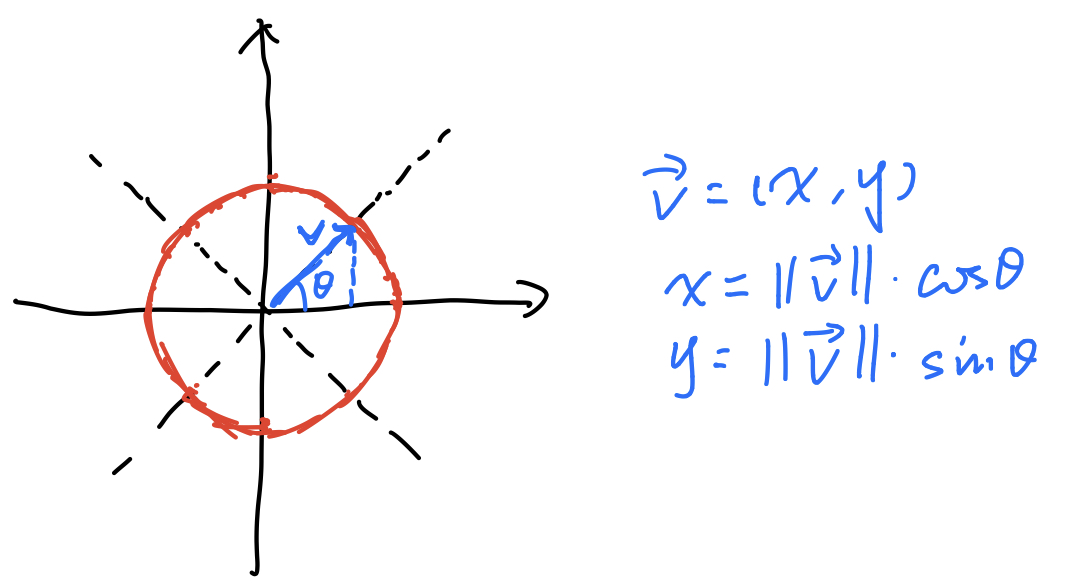
We want to span the directions uniformlly, so you know the angle , then how do you represent the vector? Simple right?
Ok so why do we need this? Remember we want to find the projection onto each of these direction vectors, and a projection is relevant to inner product right?
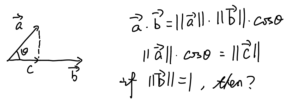
So now you have the basic idea on the concepts. In the code for this part, since it’s an inner product, where it’s essentially element-wise multiplication and summation. Does this sound familiar? You will find nn.Conv2d useful here, and remember we want to project the gradient vector onto directions, so you may convolve xxx with xxx… (I’ll leave the rest to you otherwise it’ll be like giving away the answer.)
Histogram
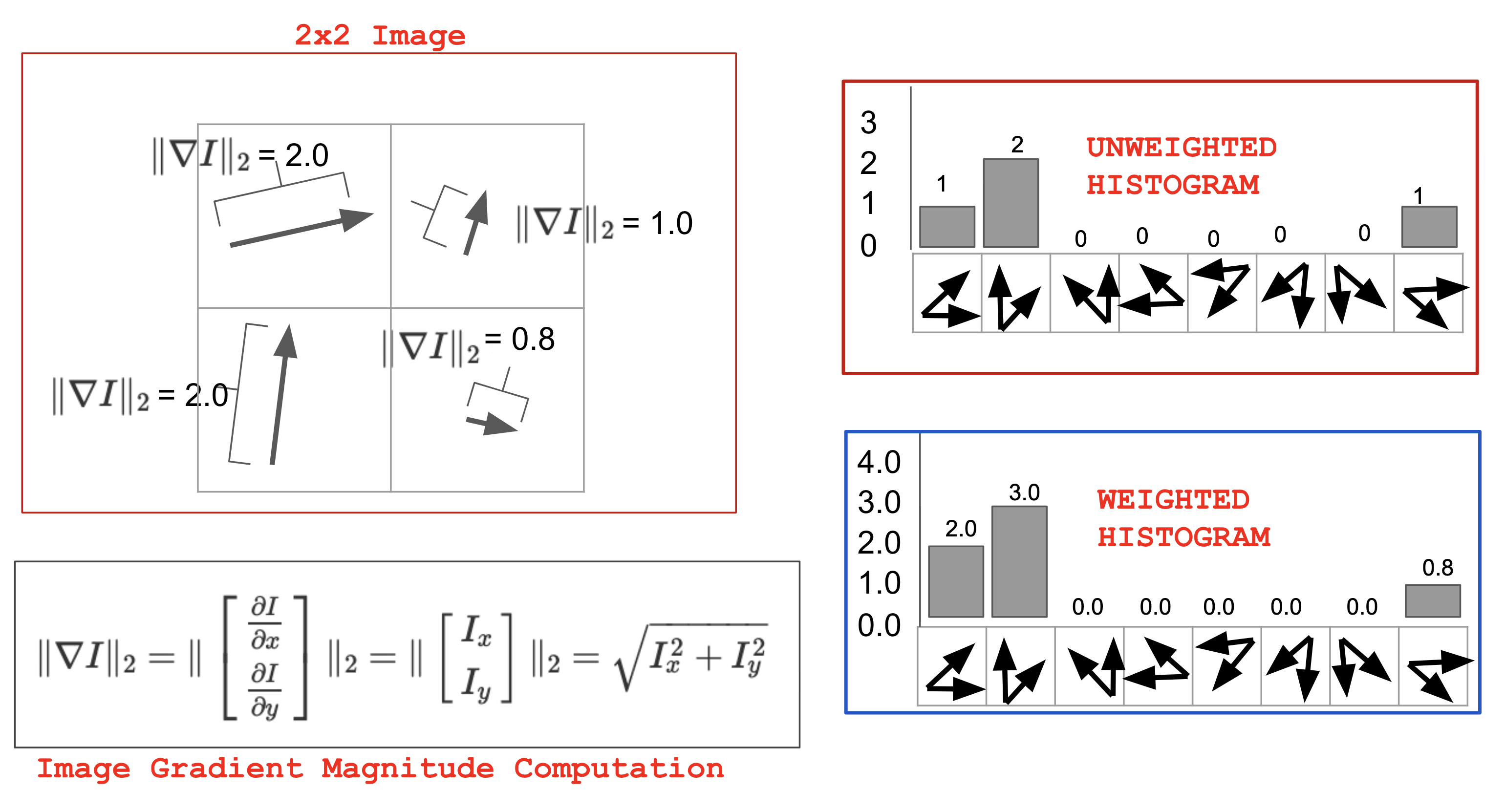
So what we want is calculating the contribution to each of the sub-regions (the figure on the Szeliski book is clearer for the idea behind this, refer to Figure 4.18 on page 224). What have we done so far? At every pixel, there are 8 values for 8 directions, and we want to calculate to which direction is this pixel contributing the most? And we’d like to assign the weight to these directions based on the magnitude of the pixel’s gradient. Check out the following figure (note that in the histogram sample, we have 8 “bins”, which correspond to what we’ve computed using projection in the previous section):
Slowest Code
To find the descriptor at every pixel, we could loop over the 16x16 patch around every pixel, then loop over the 4x4 subgrids in that 16x16 patch, then compute the gradient at every pixel.
for row:
  for column:
    for i= 0,1,2,3 for 4 neighborhoods of sz 4x4:
      for j= 0,1,2,3 for 4 neighborhoods of sz 4x4:
        for ii of 4x4 subgrid:
          for jj of 4x4 subgrid:
            for each of the 8 directions:
              if this is the direction I'm contributing the most:
                mark the magnitude
Notice that in Numpy the last line (marking the magnitude i.e. computing weighted histograms) is easy:
hist_vec, _ = np.histogram(angles, bins=8, range=(-np.pi, np.pi), weights=magnitudes)
if your orientations were all in the range , which gives you.
With 7 for-loops, this code is going to run forever. We need something much faster.
Faster Code
Notice that we are re-computing histograms over mostly shared patches. This is wasted work. Instead, we could first form a histogram at every pixel, and then just combine them over 4x4 subgrids:
Hence the most straightforward logic is to loop, loop, and loop:
for row:
  for column:
    for each of the 8 directions:
      if this is the direction Im contributing the most:
        mark the magnitude in a per-pixel histogram

for row:
  for column:
    neighborhood_histogram = zeros(8,1)
    for i = 0,1,2,3 bc subgrid of sz 4x4:
      for j= 0,1,2,3 bc subgrid of sz 4x4:
        neighborhood_histogram += per_pixel_histogram[row+i,column+j]
But as you can imagine, with 3 for-loops (and then 4 for-loops) this will still take quite long to run; that’s why you can find in the comment section that this kind of implementation will be penalized.
Even Faster Code
So think about how to speed it up. First, notice that summing over 4x4 subgrids is actually just 2d convolution. Second, notice that you can find the right bin without a for-loop – just by performing 8 dot-products with your 8-basis unit vectors around the unit circle. Last of all, a quick hint: in Numpy you can do n-dimensional array indexing with another array, like:
a = np.array([1,2,3,4,5])
idx = np.array([0,2])
print(a[idx]) # this will give you [1, 3]